TL:DR
techniques to speed up inference of LLMs to increase token generation speed and reduce memory consumption: Mixed-Precision, Bfloat16, Quantization, Fine-tuning with Adapters, Pruning, Continuous Batching and Multiple GPUs.

Companies from small startups to large corporations want to utilze the power of modern LLMs and include them into company’s products and infrastructure. One of the challenges they face is that such large models require a huge number of resources for deployment (inference). Accelerating model inference is an important challenge for developers. It is related to both the reduction of fees for computing resources and the speed of application response.
«In the future, every 1% speedup on LLM inference will have similar economic value as 1% speedup on Google Search infrastructur» — Jim Fan, NVIDIA Senior AI Scientist.
The development of LLMs and the infrastructure around them is evolving at an unthinkable rate. Every week, new approaches emerge to speed up or compress models. In such a flow of information, it’s hard to keep a finger on the pulse and have an idea of what techniques really work, not just on paper.
I tried to understand what improvements are available now for implementation in the project and how much they allow to accelerate the inference of LLM models.
“Short” Summary
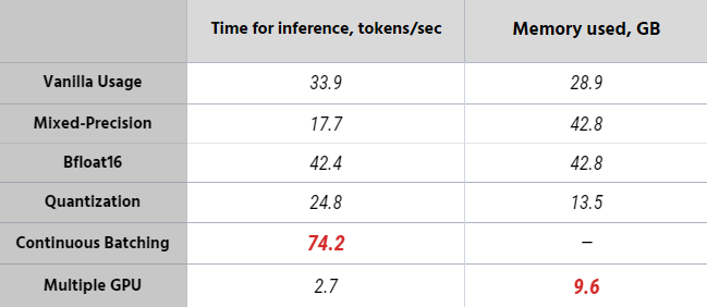
The blog post is a bit long, so there is a summary with the main points:
- Use precision reduction: float16 or bfloat16. This will speed up the model by ~20% and reduce memory consumption by 2x.
- Use 8bit or 4bit quantization to reduce memory consumption by 2x or 3x. Best for running on small devices when memory size is limited. Be careful: quantization degrades the quality of predictions.
- Use fine-tuning with adapters (LoRA, QLoRA) to improve prediction accuracy on your data. Works well in combination with quantization afterwards.
- Use Tensor Parallelism for faster inference on multiple GPUs to run large models.
- If possible, use libraries for LLM inference and serving. such as Text Generation Inference, DeepSpeed or vLLM. These already include various optimization techniques: tensor parallelism, quantization, continuous batching of incoming requests, optimized CUDA kernels, and more.
- Do some preliminary tests before using it in the production. I spent a lot of time fixing bugs in some libraries that I used. Also not all LLM have working solutions.
- Don’t forget to evaluate the final solution. It is good to have the prepared dataset for quick tests.
Let’s now discuss all these points in more detail.
Model
I decided to choose Falcon — the latest open-source large language model released by Technology Innovation Institute. It is an autoregressive decoder-only model with two variants: a 7 billion parameter model and a 40 billion parameter model. The 40B model variant was trained on 384 GPUs on AWS for 2 months.

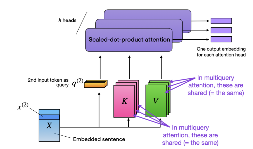
Based on what is known about the model, Falcon architecture is very similar to GPT-3 and LLaMA, except for using multiquery attention (Shazeer 2019) and RefinedWeb corpus as a training dataset (which can be a key to success).
Multiquery attention is a concept where the same key and value tensors are shared for efficiency across different attention heads, as illustrated for a multihead attention block below.
Vanilla Usage
To conduct my experiments, I used the Lit-GPT library, which includes an implementation of open-source LLM and powered by Lightning Fabric. As for the hardware setup, I used a single A100 GPU with a memory capacity of 40 GB.
To initiate experiments, the first step involves downloading the model weights and converting them to the lit-gpt format. This is quite easy to do:
python scripts/download.py --repo_id tiiuae/falcon-7b
python scripts/convert_hf_checkpoint.py --checkpoint_dir checkpoints/tiiuae/falcon-7b
To execute the model just run:
python generate/base.py \
    --prompt "I am so fast that I can" \
    --checkpoint_dir checkpoints/tiiuae/falcon-7b \
    --max_new_tokens 50 \
    --precision "32-true"

# Time for inference: 1.47 sec total, 33.92 tokens/sec
# Memory used: 28.95 GB
Methods to accelerate the LLM inference
Using 16-Bit Precision
When training deep neural networks on a GPU, we typically use a lower-than-maximum precision, namely, 32-bit floating point operations (in fact, PyTorch uses 32-bit floats by default). In floating-point representation, numbers are stored in a combination of three parts: the sign, the exponent, and the significand (or mantissa).
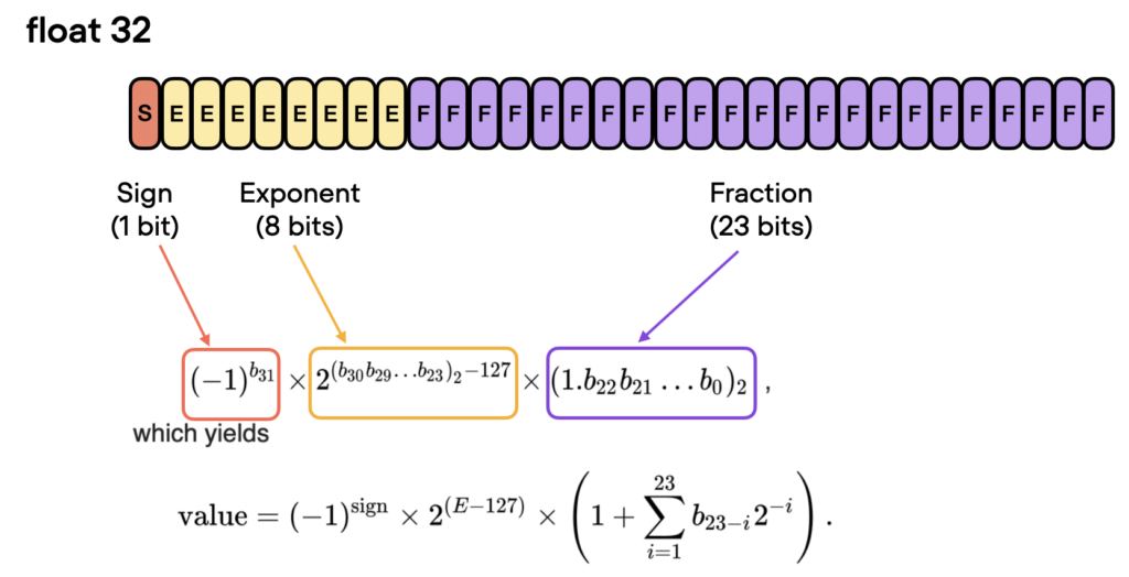
In general, a larger number of bits corresponds to a higher precision, which lowers the chance of errors accumulating during computations. However, if we want to speed up our model, we can reduce the precision to, for example, 16-bit precision. How this can help:
- Reduced memory size. 32-bit precision requires twice as much GPU memory as 16-bit precision, allowing more efficient use of GPU memory.
- Increased compute and speed. Since operations on lower precision tensors require less memory, GPUs can process them more quickly.
Lit-GPT uses the Fabric library, which allows to change the precision in a few lines of code.
python generate/base.py \
    --prompt "I am so fast that I can" \
    --checkpoint_dir checkpoints/tiiuae/falcon-7b \
    --max_new_tokens 50 \
    --precision "16-true"

# Time for inference: 1.19 sec total, 42.03 tokens/sec
# Memory used: 14.50 GB
Mixed-Precision Training
Mixed-precision training is one of the essential techniques that lets us significantly boost training speeds on modern GPUs. We don’t transfer all parameters and operations to 16-bit floats. Instead, we switch between 32-bit and 16-bit operations during training, hence, the term “mixed” precision.

This approach allows for efficient training while maintaining the accuracy and stability of the neural network.
python generate/base.py \
    --prompt "I am so fast that I can" \
    --checkpoint_dir checkpoints/tiiuae/falcon-7b \
    --max_new_tokens 50 \
    --precision "16-mixed"

# Time for inference 1: 2.82 sec total, 17.70 tokens/sec
# Memory used: 42.84 GB
Brain Floating Point
Bfloat16 is a floating-point number format proposed by Google. The name stands for “Brain Floating Point Format” and it originates from the Google Brain artificial intelligence research group at Google. Here you can read more about the Bfloat16 Arithmetic.
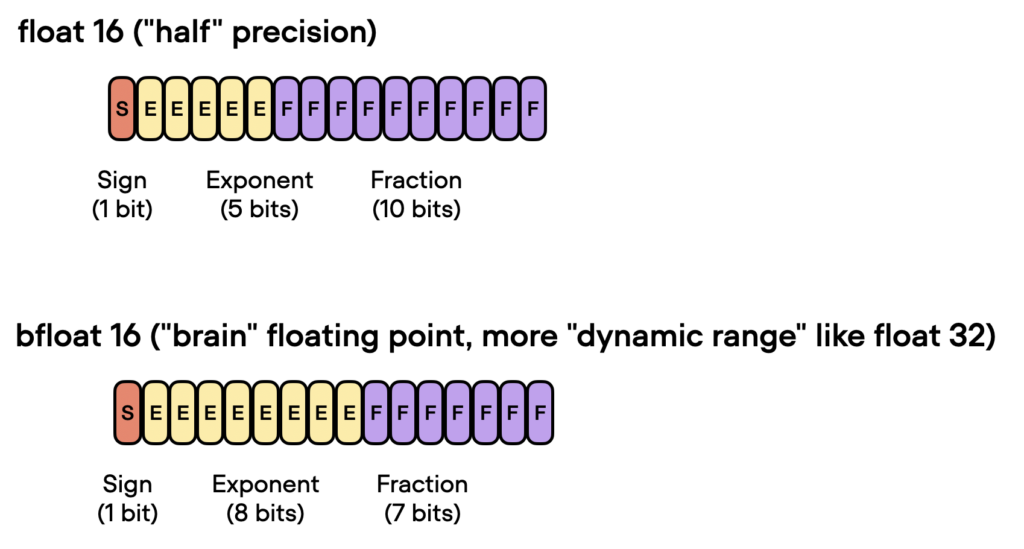
Google developed this format for machine learning and deep learning applications, particularly in their Tensor Processing Units (TPUs). While bfloat16 was originally developed for TPUs, this format is now supported by several NVIDIA GPUs as well.
You can check whether your GPU supports bfloat16 via the following code:
python -c "import torch; print(torch.cuda.is_bf16_supported())"
If you have bfloat support, you can run the following command:
python generate/base.py \
    --prompt "I am so fast that I can" \
    --checkpoint_dir checkpoints/tiiuae/falcon-7b \
    --max_new_tokens 50 \
    --precision "bf16-true"

# Time for inference: 1.18 sec total, 42.47 tokens/sec
# Memory used: 14.50 GB
The results from above are summarized in the following chart:

Quantization
If we want to increase the model performance during inference even more, we can also move beyond lower floating point precision and use quantization. Quantization converts the model weights from floats to low-bit integer representations, for example, 8-bit integers (and, recently, even 4-bit integers).
There are two common approaches for applying quantization on a deep neural network:
- Post-Training Quantization (PTQ): A model is first trained to convergence and then we convert its weights to lower precision without more training. It is usually quite cheap to implement, in comparison to training.
- Quantization-Aware Training (QAT): Quantization is applied during pre-training or further fine-tuning. QAT is able to attain better performance but requires extra computation resources and access to representative training data. Since we want to speed up an existing model, we will use Post-Training Quantization. You can read more about different techniques of post-training quantization here.
NOTE: A research paper published recently, SmoothQuant: Accurate and Efficient Post-Training Quantization for Large Language Models has shown that not all quantization techniques effectively work with large language models (LLMs). Therefore, give attention to the quantization approach that you will use. Personally, I would advise you to pay attention to this article SpQR: A Sparse-Quantized Representation for Near-Lossless LLM Weight Compression, which explores LLAMA and Falcon quantization.
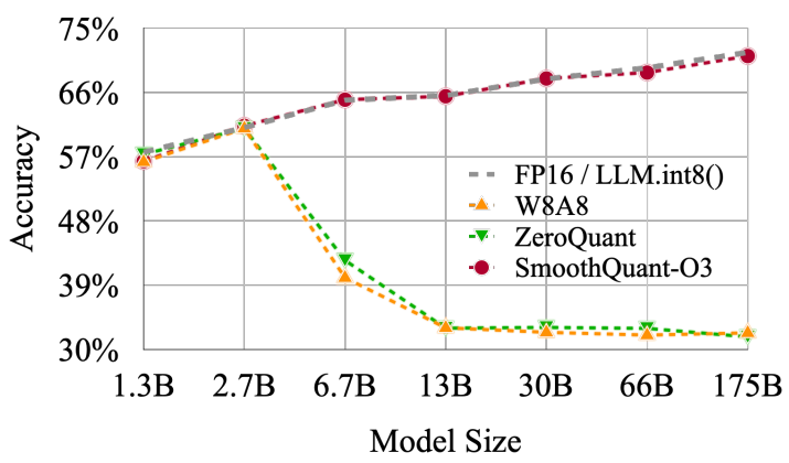
Since 4bit and 8bit precision for Falcon models is not implemented yet, I will show an example with LLaMA 7B using Lit-LLaMA.
python generate.py \
    --prompt "I am so fast that I can" \
    --quantize llm.int8

# Time for inference: 2.01 sec total, 24.83 tokens/sec
# Memory used: 13.54 GB
Fine-tuning with adapters
While fine-tuning may not be a direct method for expediting the inference process of the final model, there are a few tricks that can be employed to optimize its performance:
- Pre-training and Quantization: Start by pre-training your model on the specific domain problem and then proceed to quantize it. Quantization typically leads to a slight decrease in model quality, but this can be mitigated by the initial pre-training.
- Small Adapters: Another approach involves incorporating small adapters for different tasks. Adapters operate by adding compact additional layers to the existing model layers and solely training them. These adapter layers have lightweight parameters, enabling the model to rapidly adapt and learn.
Using these methods in combination, you can increase the effectiveness of your model.
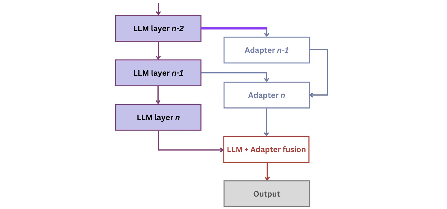
Within the realm of adapters, several variations have emerged, including LLaMA-Adapter (v1, v2), LoRa, and QLoRa. Among these, Low-Rank Adaptation (LoRA) stands out prominently. LoRA introduces a minuscule number of trainable parameters, referred to as adapters, to each layer of the LLM. Simultaneously, it freezes all the original parameters. This approach simplifies the fine-tuning process by updating only the adapter weights, which significantly reduces memory consumption.
The QLoRA approach, which added quantization and a few other optimizations to LoRA, revolutionized the way we can fine-tune a model on a Google Colab instance!
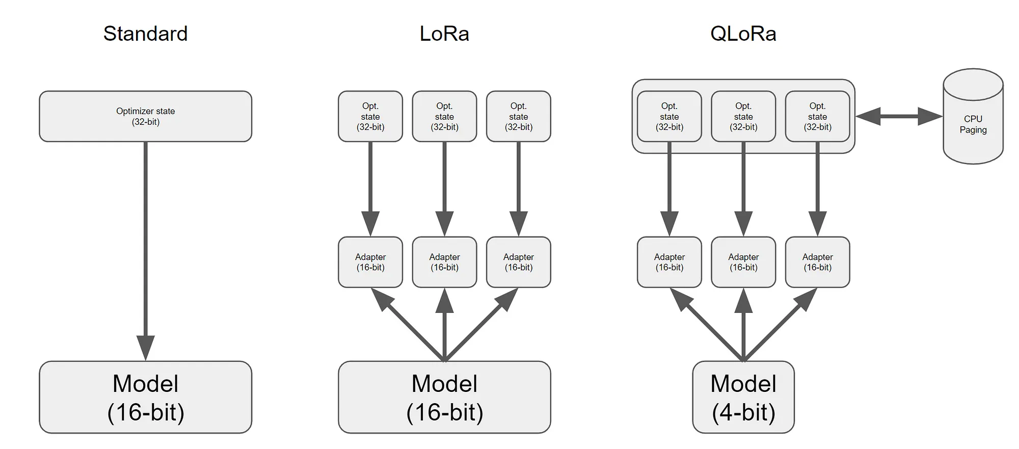
Fine-tuning an LLM can be a resource-intensive process, entailing a considerable investment of time and computational power. For instance, fine-tuning Falcon-7B can take around half an hour when executed on 8 A100 GPUs or approximately 3 hours when using a single GPU. In addition, optimal results require proper preparation of the dataset. While I haven’t personally performed the fine-tuning process for the model, if you wish to embark on it yourself, you can initiate the procedure by running the following command (read more about it here):
python finetune/adapter_v2.py \
    --data_dir data/alpaca  \
    --checkpoint_dir checkpoints/tiiuae/falcon-7b \
    --out_dir out/adapter/alpaca
For further details and in-depth information, I recommend the following resources:
- Understanding Parameter-Efficient Finetuning of Large Language Models: From Prefix Tuning to LLaMA-Adapters
- Making LLMs even more accessible with bitsandbytes, 4-bit quantization and QLoRA
- Finetuning Falcon LLMs More Efficiently With LoRA and Adapters
- Colab notebook to fine-tune Falcon-7B on Guanaco dataset using 4bit and PEFT
Pruning
Network pruning is to reduce the model size by trimming unimportant model weights or connections while the model capacity remains.
New method LLM-Pruner adopts structural pruning that selectively removes non-critical coupled structures based on gradient information, maximally preserving the majority of the LLM’s functionality. Authors demonstrate that the compressed models still exhibit satisfactory capabilities in zero-shot classification and generation.

The authors of the article have posted the code, but supported LLMs are only LLaMA-7B and Vicuna-7B.
Other interesting pruner — Wanda (Pruning by Weights and activations). This approach prune weights with the smallest magnitudes multiplied by the corresponding input activations, on a per-output basis.

Notably, Wanda requires no retraining or weight update, and the pruned LLM can be used as is. Also it allows prune LLMs to 50%.
Batch Inference
GPUs, renowned for their massively parallel compute architectures, boast astounding compute rates measured in teraflops (floating-point operations per second) for models such as the A100, and even petaflops for models like the H100. Despite the immense computational power available, LLMs often struggle to fully exploit the potential due to a significant portion of the chip’s memory bandwidth being consumed by loading model parameters.
One effective approach to mitigate this limitation is through batching. Instead of loading new model parameters for every input sequence, batching allows for loading the parameters once and utilizing them to process multiple input sequences. This optimization strategy efficiently utilizes the chip’s memory bandwidth, resulting in higher compute utilization, improved throughput, and more cost-effective LLM inference. By employing batching techniques, the overall performance of LLMs can be significantly enhanced.
One recent such proposed optimization is continuous batching. Instead of waiting until every sequence in a batch has completed generation, Orca implements iteration-level scheduling where the batch size is determined per iteration. The result is that once a sequence in a batch has completed generation, a new sequence can be inserted in its place, yielding higher GPU utilization than static batching.

There are several frameworks where you can use this algorithm:
- Text Generation Inference — server for text generation inference.
- vLLM — inference and serving engine for LLMs.
After careful evaluation, I personally opted for vLLM as my preferred choice. vLLM utilizes PagedAttention, the new attention algorithm that effectively manages attention keys and values: it delivers up to 24x higher throughput than HuggingFace Transformers, without requiring any model architecture changes.

Considering the unavailability of support for Falcon within vLLM, I made the decision to utilize LLaMA-7B instead.
from vllm import LLM, SamplingParams


prompts = [
    "I am so fast that I can",
    "The capital of France is",
    "The future of AI is",
]
sampling_params = SamplingParams(temperature=0.8, top_p=0.95)
llm = LLM(model="huggyllama/llama-7b")
outputs = llm.generate(prompts, sampling_params)

for output in outputs:
    prompt = output.prompt
    generated_text = output.outputs[0].text
    print(f"Prompt: {prompt!r}, Generated text: {generated_text!r}")


# I am so fast that I can travel around the world in two hours. My first stop: the Southeast
# The capital of France is one of the most beautiful cities in the world. And it is no secret that
# The future of AI is in a future\nThis might sound like a depressing conclusion, but it
I was thoroughly impressed by the remarkable speed at which it operated. Moreover, the framework facilitated the seamless setup of the API server, enabling swift deployment. To initiate the process, simply execute the following command
python -m vllm.entrypoints.api_server --model huggyllama/llama-7b
Then you can check the functionality:
time curl http://localhost:8000/generate \
    -d '{
        "prompt": "I am so fast that I can",
        "temperature": 0,
        "use_beam_search": true,
         "n": 4,
    }'

# 🚀 real    0m0.277s
# I am so fast that I can take through a story three get back before I started.
# I am so fast that I can turn around a Earth in come back for lunch.
# I am so fast that I can finish on the earth, still be for lunch.\nI am so fast
# I am so fast that I can run around the world and grab my own feet start.
You can find a more detailed review and benchmarks of Batch Inference here.
Multiple GPU devices
You can also use the Fully-Sharded Data Parallel (FSDP) distributed strategy to leverage multiple devices to perform inference. It is important to understand that using ultiple GPU devices does not speed up inference, but allows you to run models that wouldn’t fit in a single card by sharding them across several.
For instance, falcon-40b would require ~80 GB of GPU memory to run on a single device. We can instead run it on 2x A6000 (48 GB) still using Lit-GPT, adding just a few parameters:
python generate/base.py \
    --checkpoint_dir checkpoints/tiiuae/falcon-40b \
    --strategy fsdp \
    --devices 2 \
    --prompt "I am so fast that I can"

# Time for inference: 83.40 sec total, 0.60 tokens/sec
# Memory used: 46.10 GB
Which will take 46 GB of memory, and run at 0.60 tokens/sec.

Alternatively, we have the option to use vLLM, which generates text much faster simply by setting tensor_parallel_size to 2.
prompts = [
    "I am so fast that I can",
    "The capital of France is",
    "The future of AI is",
]
llm = LLM(model="huggyllama/llama-30b", tensor_parallel_size=2)
output = llm.generate(prompts, sampling_params)


# 🚀 It takes only 0.140 seconds!
# I am so fast that I can travel back in time and eat my breakfast before I eat my breakfast!
# The future of AI is up to you.
Bonus section: Serving LLM models
Since vLLM does not support Falcon, I decided to show how you can easily deploy a model using Text Generation Inference.
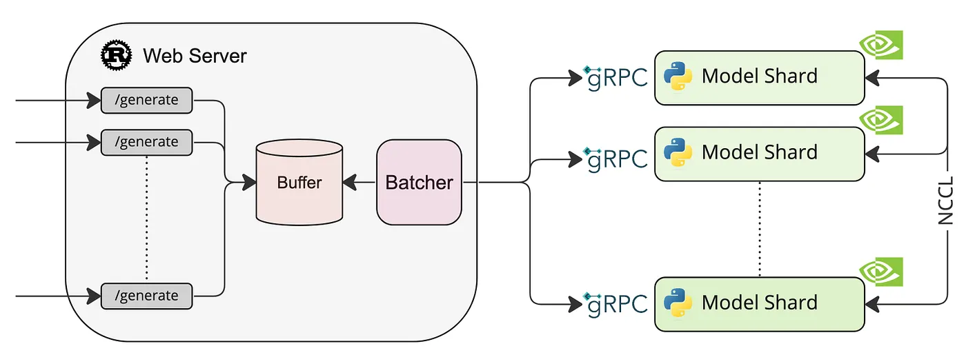
To adhere to the recommended best practices of the framework’s authors, it is advisable to execute the provided command and run the application within a Docker container. Run the docker container:
docker run --gpus all --shm-size 1g -p 8080:80 \
    -v $PWD/data:/data ghcr.io/huggingface/text-generation-inference:0.8 \
    --model-id tiiuae/falcon-40b --num-shard 1 --quantize bitsandbytes
Please take note that Falcon-7B does not support tensor parallelism. Consequently, it is crucial to set the parameter num_shard to 1 to ensure proper functionality.
During my own experience, the process involved approximately 2 minutes to download the Docker image, followed by 30 seconds to download the scales. Subsequently, it took roughly 20 seconds to convert the scales from the .bin format to .safetensors. Finally, the download of the final model required approximately 1 minute to complete. These time estimates provide an overview of the duration of these specific steps in the process.
You can check API with the following command:
time curl http://localhost:8080/generate \
     -X POST \
     -d '{"inputs":"I am so fast that I can","parameters":{"max_new_tokens":50}}' \
     -H 'Content-Type: application/json'


# real    0m3.148s
# I am so fast that I can do two things at the same time.
Other alternative libraries for the LLM Inference:
- Accelerate let you offload part of the model onto the CPU. Offloading helps you optimize the throughput of an inference service, even when the whole model fits on a GPU.
- DeepSpeed Inference helps you serve transformer-based models more efficiently when: (a) The model fits on a GPU, and (b) The model’s kernels are supported by the DeepSpeed library. This is your go-to solution if latency is your main concern.
- DeepSpeed MII is a library that quickly sets up a GRPC endpoint for the inference model, with the option to use either the ZeRO-Inference or DeepSpeed Inference technology.
- OpenLLM is an open platform for operating large language models (LLMs) in production. Fine-tune, serve, deploy, and monitor any LLMs with ease.
- Aviary — a new open source project that simplifies and enables easy self-hosted serving of multiple LLM models efficiently
Reed more about them here.
Conclusions
The field of LLM acceleration is a complex landscape that is still in its infancy. In the course of preparing this article, I encountered numerous recently developed methods, some of which have shown promising potential (appeared within the last 1–2 months).
However, it is important to note that not all acceleration methods work without compromise. Some methods may degrade the quality of the model. Consequently, it is unwise to blindly accept and apply all acceleration advice without careful consideration. You must remain vigilant in controlling the quality of the accelerated model.
Ideally, achieving a balance between software optimization and model architecture is the key to achieving efficient LLM acceleration.